Differential evolution (DE) is a more recent stochastic population-based evolutionary method introduced by Storn and Price [1] in 1996. It follows the standard evolutionary algorithm flow with some significant differences in mutation and selection process. The simplicity of DE algorithm is based on only two tunable parameters, the mutation factor $F$ and the crossover probability $CR$. The fundamental idea behind DE is the use of vector differences by choosing randomly selected vectors, and then taking their difference as a means to perturb the parent vector with a special kind operator and probe the search space. Several variants of DE have been proposed so far [2, 3], but the following analysis is focused on the nominal approach (DE/rand/1/bin). According to this, each of the members of the population undergoes mutation and crossover. Once crossover occurs, the offspring is compared to the parent, and whichever fitness is better is moved to the next generation (selection) (see Fig. 1).
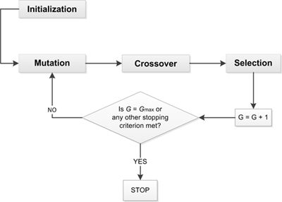
Figure 1: Differential evolution process.
Mutation
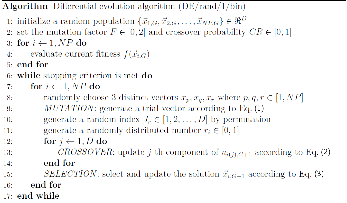
After initialization each of the members of the population undergoes mutation and a donor vector $\vec{v}_{i, G + 1}$ is generated such as: \begin{equation} \vec{v}_{i, G + 1} = \vec{x}_{p, G} + F \cdot (\vec{x}_{q, G} - \vec{x}_{r, G}) \label{eq:mutation} \end{equation} $G$ is current generation, $NP$ is the population size and $F$ is a real constant value, called the mutation factor. Integers $p$, $q$ and $r$ are chosen randomly from the interval $[1, NP]$ while $x_{i, G} \neq x_{p, G} \neq x_{q, G} \neq x_{r, G}$.
Crossover
In the next step the crossover operator is applied by generating the trial vector $\vec{u}_{i(j), G + 1}$ which is defined from the $j$-th component of $\vec{x}_{i(j), G}$ or $\vec{v}_{i(j), G + 1}$ with probability $CR$: \begin{equation} \begin{aligned} u_{i(j), G + 1} &= \left\{ \begin{array}{ll} v_{i(j), G + 1} \mbox{, } & \text{if} \;\; r_{i} \leq CR \;\; \text{or} \;\; j = J_{r} \\ x_{i(j), G} \mbox{, } & \text{if} \;\; r_{i} > CR \;\; \text{or} \;\; j \ne J_{r} \end{array} \right. \\ \{i, j \} &= 1, 2, \dots, NP \end{aligned} \label{eq:crossover} \end{equation} where $r_{i} \sim U[0, 1]$ and $J_{r}$ is a random integer from $[1, 2, \dots, D]$ which ensures that $\vec{v}_{i, G + 1} \neq \vec{x}_{i, G}$. $D$ is the problem dimension.
Selection
The last step of the generation procedure is the implementation of the selection operator where the vector $\vec{x}_{i, G}$ is compared to the trial vector $\vec{u}_{i, G + 1}$: \begin{equation} \begin{aligned} \vec{x}_{i, G + 1} &= \left\{ \begin{array}{ll} \vec{u}_{i, G + 1} \mbox{, } & \text{if} \;\; f(\vec{u}_{i, G + 1}) \leq f(\vec{x}_{i, G}) \\ \vec{x}_{i, G} \mbox{, } & \text{otherwise} \end{array} \right. \\ i &= 1, 2, \dots, NP \end{aligned} \label{eq:selection} \end{equation} where $f(\vec{x})$ is the objective function to be optimized, while without loss of generality the implementation described in Eq. (\ref{eq:selection}) corresponds to a minimization problem. The whole process is summarized in the following algorithm:
References
- Storn R. and Price K. (1997). Differential evolution - a simple and efficient heuristic for global optimization over continuous spaces. Journal of Global Optimization, 11(4), 341-359.
- Price K., Storn R. M., and Lampinen J. A. (2005). Differential Evolution - A Practical Approach to Global Optimization. Springer.
- Das S. and Suganthan P. (2011). Differential evolution: A survey of the state-of-the-art. IEEE Transactions on Evolutionary Computation, 15(1):4-31, 2011.